Greedy algorithms - Part 2

This page is the second of a series of short tutorials on topics covered by the upcoming book Intelligent Optimization - Optimization plus Machine Learning for Reliable Artificial Intelligence by Roberto Battiti, Kevin Tierney and Mauro Brunato.

This tutorial is released under the Creative Commons Attribution-NonCommercial-ShareAlike 4.0 International license (CC BY-NC-SA 4.0)

Prerequisites

We need the packages already installed during at the beginning of the first tutorial. Furthermore, to get a better view of our problem instance, we install the SciPy package:

!pip install scipy

We also need some of the objects and functions that we created in the first tutorial, so we created the package Code.greedy_algorithms_1 containing the relevant definitions. As usual, we will import every definition when we need it.

A (still greedy) alternative

Remember the main drawback from the previous greedy heuristic? As the vehicle wandered farther from its home depot, it had to skip more and more clients because it didn’t have the residual capacity to serve them. As a result, depots “stole” clients to each other.

Let us add the constraint that every client must be served by its closest depot. To do so, let us split the clients based on their distances from the depots and apply the previous greedy construction separately to each domain.

Visualizing the Voronoi diagram

First of all, we can use the scipy.Voronoi class to visualize the Voronoi diagram of the depots, useful to (visually, at least) identify the closest depot to every client by dividing the plane into their proximity domains.

The following function returns the Voronoi diagram object for the set of depots in a problem instance:

import numpy as np
from scipy.spatial import Voronoi, voronoi_plot_2d
import pyvrp

def get_Voronoi_diagram(data: pyvrp.ProblemData) -> Voronoi:
    # Organize the depot coordinates into a (num_depots x 2) matrix
    depot_points = np.array([
        [data.location(i).x, data.location(i).y]
        for i in range(data.num_depots)
    ])
    # Compute and return the Voronoi diagram
    return Voronoi(depot_points)

At this point, we can write a small helper function to visualize the diagram and, if needed, superimpose it to the pyvrp plot (that’s why we have an optional axis, so that we can draw the diagram on an existing chart):

from typing import Optional
import matplotlib.pyplot as plt

def plot_Voronoi_diagram(vor: Voronoi, ax: Optional[plt.Axes] = None) -> None:
    # draw the Voronoi diagram on the existing axis
    # (if any) without additional elements
    voronoi_plot_2d(vor, ax=ax, show_points=False, show_vertices=False)
    # Restore the original x and y limits
    plt.xlim(-20,120)
    plt.ylim(0,100)

Finally, we can see how the clients can be partitioned among the depots:

# Let us use the same problem instance from the previous tutorial:
from Code.greedy_algorithms_1 import model

ax = plt.axes()
vor = get_Voronoi_diagram(model.data())
plot_Voronoi_diagram(vor, ax)
pyvrp.plotting.plot_coordinates(model.data(), ax=ax)
_=ax.legend([])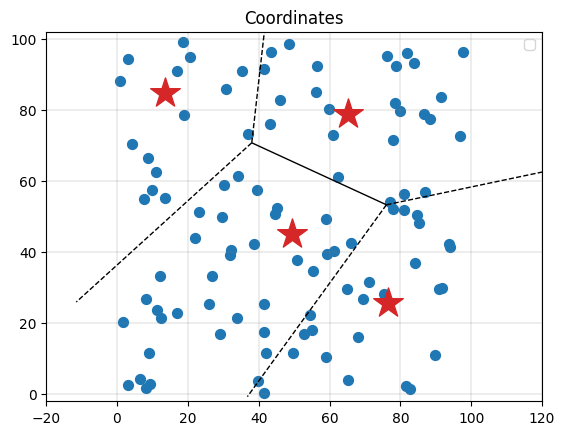

Finding the closest depot to a client

Let’s now put this idea into practice: first, a helper function that returns the closest depot to an arbitrary client.

Arguments:
- data the problem instance data, in particular the distance matrix
- client_index the index of the client whose closest depot we are looking for
Return value:
- the index of the closest depot.

def closest_depot(data: pyvrp.ProblemData, client_index: int) -> int:
    # retrieve the full distance matrix
    distance_matrix = data.distance_matrix(0)
    # initialize the (currently) closest depot and distance
    best_distance = 10000000
    depot_index: Optional[int] = None
    # scan all depots and replace the current closest if needed
    for i in range(data.num_depots):
        d = distance_matrix[i, data.num_depots+client_index]
        if depot_index is None or d < best_distance:
            best_distance = d
            depot_index = i
    # return the closest depot
    assert depot_index is not None
    return depot_index

The new greedy function

The construction of the solution is very similar to the previous one, but first it partitions the set of clients among the depots, and during its operation it maintains a set of unserved clients for each depot.

Arguments:
- data the problem instance data;
- update_callback: as in previous construction functions, an optional callback to be invoked every time a new client is added to the current route, used to animate the greedy construction - as usual, you can safely ignore its existence.
Returns:
- the full solution

# To build a single route we use the same function defined in the previous tutorial
from Code.greedy_algorithms_1 import build_greedy_route

from typing import Callable
def build_greedy_closest_depot_solution(
    data: pyvrp.ProblemData,
    update_callback: Optional[Callable[[pyvrp.Solution], None]] = None
) -> pyvrp.Solution:
    # list of greedy routes, used to build the solution object after it's filled up
    greedy_routes: list[pyvrp.Route] = []
    # partition the set of available clients for each depot
    unserved_clients: list[set[int]] = [set() for _ in range(data.num_depots)]
    for client_index in range(data.num_clients):
        unserved_clients[closest_depot(data, client_index)].add(client_index)
    # For every depot:
    for depot_index in range(data.num_depots):
        # repeat until there are no more clients in the depot-specific set
        while len(unserved_clients[depot_index]) > 0:
            # get the next greedy route starting from the chosen depot
            route = build_greedy_route( # from the 1st tutorial
                data,
                unserved_clients[depot_index],
                depot_index,
                # if the callback is defined, create a partial solution with the
                # current routes and invoke it
                None if update_callback is None
                else lambda partial_route:
                    update_callback(
                        pyvrp.Solution(data, greedy_routes + [partial_route])
                    )
                )
            # create the corresponding Route object and append it
            # to the list of routes
            greedy_routes.append(route)
    # Create the solution object and return it
    return pyvrp.Solution(data, greedy_routes)

Now we can build the new greedy solution. First of all, let’s rewrite the callback function of the previous tutorial to add the Voronoi diagram:

from IPython.display import display, clear_output
from time import sleep

def solution_callback_with_voronoi_diagram(partial_solution: pyvrp.Solution) -> None:
    # clear the current output
    clear_output(wait=True)
    # forget the current plot
    plt.close()
    # plot the solution on the current axis
    ax = plt.axes()
    plot_Voronoi_diagram(vor, ax)
    pyvrp.plotting.plot_solution(
        partial_solution, model.data(), ax=ax, plot_clients=True
    )
    # No legend
    ax.legend([])
    # Actually show the plot and wait a short time
    display(plt.gcf())
    sleep(.01)

Finally, we can test our strategy!

For the animation to work properly, we must get rid of an annoying message issued by Matplotlib, therefore we temporarily reroute the standard error stream to a file:

# Reroute the standard error stream
import sys
old_stderr = sys.stderr # keep the old reference
sys.stderr = open('warnings.log', 'w')
# Compute the solution
greedy_closest_depot_solution = build_greedy_closest_depot_solution(
    model.data(),
    solution_callback_with_voronoi_diagram
)
plt.close()
# Restore the standard error stream
sys.stderr = old_stderr

Analysis of the result

Did we improve the result? On first glance it seems to be the case. Here are the two solutions side by side, together with the (better) solution found by pyvrp’s CP solver.

from Code.greedy_algorithms_1 import cp_solution, greedy_solution

_, axes = plt.subplots(figsize=(13,4), ncols=3, sharey=True)
pyvrp.plotting.plot_solution(cp_solution.best, model.data(), ax=axes[0])
axes[0].set_title(f'CP ({cp_solution.best.distance()})')
_=axes[0].legend([])
pyvrp.plotting.plot_solution(greedy_solution, model.data(), ax=axes[1])
axes[1].set_title(f'1st greedy heuristic ({greedy_solution.distance()})')
_=axes[1].legend([])
pyvrp.plotting.plot_solution(greedy_closest_depot_solution, model.data(), ax=axes[2])
axes[2].set_title(f'2nd greedy heuristic ({greedy_closest_depot_solution.distance()})')
_=axes[2].legend([])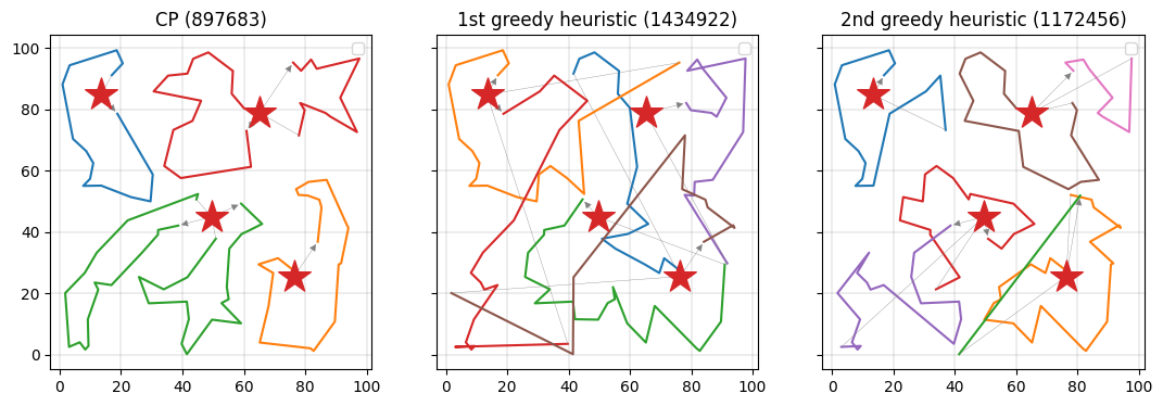

In particular, let’s quantify the improvement:

improvement = (greedy_solution.distance() - greedy_closest_depot_solution.distance()) / greedy_solution.distance()
print(f'The 2nd greedy solution is shorter than the 1st by {improvement*100:.0f}%.')
gap_to_cp = (greedy_closest_depot_solution.distance() - cp_solution.best.distance()) / cp_solution.best.distance()
print(f'It is still worse than the CP solution by {gap_to_cp*100:.0f}%.')

The 2nd greedy solution is shorter than the 1st by 18%.
It is still worse than the CP solution by 31%.

Now what?

Although better greedy strategies can yield significant improvements, let us not forget that VRP is a well-known NP-hard problem. As such, we cannot expect such simple strategy to achieve an optimal result.

In the following installments, we shall try to refine these initial solutions by various local search optimization strategies, where “local moves” (such as assigning a client to a different route) are employed to gradually improve the overall solution.