Bayesian Optimization

This page is part of a series of short tutorials on topics covered by the book Intelligent Optimization - Optimization meets Machine Learning by Roberto Battiti, Kevin Tierney and Mauro Brunato.

This tutorial is released under the Creative Commons Attribution-NonCommercial-ShareAlike 4.0 International license (CC BY-NC-SA 4.0)

A Gaussian process in action

Prerequisites

To experiment this notebook locally, you must have at least one of the following:

a working Jupyter notebook server on your computer
access to a remote notebook server (i.e., Google Colabs);
a suitable local editor (e.g., Visual Studio Code with the appropriate extension).

To set up all necessary packages in your environment, the following installation command only needs to be run once.

Our purpose is to build a Bayesian Optimization framework from scratch, thus we aren’t going to use any Bayesian optimization specific package.

!pip install numpy scipy matplotlib

The Context

We have a real-valued function of \(d\) real variables:

\[ f: D\to{\mathbb R}\qquad\text{where}\qquad D\subset{\mathbb R}^d. \]

We can make very general assumptions on this function, e.g.:

it may be stochastic (i.e., its evaluation is subject to some noise);
we do not have an explicit formula - we can only evaluate it (it’s a “black box”);
it can be very costly to evaluate, therefore we should keep our evaluations to a minimum.

Our objective is to minimize \(f\), i.e., find \(x^*\in D\) such that \(f(x^*)=\min_{x\in D}f(x)\).

While our code works for any number of dimensions, as an example we will use a simple 1-dimensional real function with no noise:

\[\begin{eqnarray*} f: [-1,1] &\to& {\mathbb R}\\ x &\mapsto& \sin 7x \cdot (1-\tanh 2x^2). \end{eqnarray*}\]

Let us define it in code. Even if in our case the argument is scalar, we still represent it with a numpy array to enable the transition to multiple dimensions:

import numpy as np
def f(x: np.ndarray) -> np.float64:
    return np.sin(7*x[0]) * (1 - np.tanh(2*x[0]**2))

Let’s have a look at our function. Let us define a 400-point grid X that we shall use throughout this tutorial for plotting purposes and a corresponding array of function values f_X:

X = np.linspace(-1, 1, 400)
# every element of X is a numpy float64 number,
# we need to reinterpret it as a size-i array to pass it to f
f_X = [f(x_i.reshape(1)) for x_i in X]

Next we ca plot the two arrays:

from matplotlib import pyplot as plt
# Resize the figure in order to better fit the page
plt.figure(figsize=(12,5))
plt.plot(X, f_X)
plt.xlabel('$x$')
plt.ylabel('Target function value $f(x)$')
plt.grid()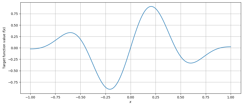

So \(f\) has two local minima, slightly above .25 and .5, the first being the global minimum we look for.

A Gaussian Process Primer

Given the assumptions on \(f\), mainly its computational hardness, our main target is to generate a surrogate of this function with the aim of representing our knowledge about it; this surrogate will be initialized with some prior assumptions (if any) and will be updated as long as new information is gathered by evaluations. In particular, the surrogate should possess the following properties:

its domain should include that of \(f\);
it should be faster to evaluate with respect to the original function;
it should summarize what we know about \(f\), associating an expected value and an uncertainty measure at each point.

In other words, we want to define a “parametric” real-valued distribution, whose parameters have values in \(D\). Since we will assume that the distribution is normal, what we want to define is a Gaussian process \({\mathcal F}\):

\[\begin{eqnarray*} {\mathcal F}: D &\to& {\mathcal D}({\mathbb R})\\ x &\mapsto& {\mathcal N}(\mu(x), \sigma(x)) \end{eqnarray*}\]

where the mean value \(\mu\) and rms \(\sigma\) depend on \(x\).

Before even evaluating the function once, we may assume that we have some prior knowledge about \(f\) in form of an initial mean value \(\mu_0(x)\) for every \(x\in D\).

Let us define a data PriorFunction type or the prior, which is a generic function mapping a numpy array into a real value:

from typing import Callable
PriorFunction = Callable[[np.ndarray], np.float64]

The only other assumption in order to build a sound model out of a set of sample evaluations is a function \[ \Sigma: D\times D \to {\mathcal R} \] that returns the expected covariance of the random variables associated to two evaluation points. The rationale is that closer points are expected to have a high covariance, while points that are father apart are more and more independent (but other dependencies are possible if, e.g., the modeled function is periodic).

The function \(\Sigma\) is thus called the “covariance function”, or “kernel”, of the Gaussian process. A reasonably simple definition is the so-called “Radial basis function” (RBF) which considers a quadratic exponential decay with distance:

\[ \Sigma(x,x') = e^{\displaystyle-\frac{\|x-x'\|^2}{2\ell^2}} \]

where \(\ell\) is a scaling factor (aka the “characteristic length” of the process).

Let us define the CovarianceFunction type:

CovarianceFunction = Callable[[np.ndarray, np.ndarray], np.float64]

These are all the assumptions we need. Let us now define a class to manage the Gaussian process.

The class GaussianProcess will need to maintain a few objects in it:

the search space dimension (\(d\) in the formulas above);
a list of sample points, which will be updated as the target function is evaluated at more and more points;
a numpy array containing the corresponding sample values;
a matrix containing the correlation function computed between each pair of sample points; this matrix will be fundamental to evaluate the model;
the inverse of the same matrix (to simplify the computations);
the covariance function;
the prior function.

Let us start by writing the constructor to initialize the class.

class GaussianProcess:
    # Number of independent variables in the domain
    dimension: int
    # list of sample points in the domain
    sample_points: list[np.ndarray]
    # corresponding array of function values at the sample points
    sample_values: np.ndarray
    # covariance between pairs of sample points
    covariance_matrix: np.ndarray
    # inverse of the above matrix
    inverted_covariance_matrix: np.ndarray
    # prior function knowledge mu_0(x)
    prior_function: PriorFunction
    # assumed covariance function between pairs of points in D
    covariance_function: CovarianceFunction
    # Constructor: build an empty model
    def __init__(
        self,
        dimension: int,
        prior_function: PriorFunction,
        covariance_function: CovarianceFunction
    ) -> None:
        self.dimension = dimension
        # No sample points
        self.sample_points = []
        # 0-element array of sample values
        self.sample_values = np.empty(0)
        # 0x0 covariance matrix
        self.covariance_matrix = np.empty((0,0))
        # provided prior and covariance functions
        self.prior_function = prior_function
        self.covariance_function = covariance_function

Next, let us define the function that adds a freshly evaluated sample point to the process.

Arguments:

x is the point in \(D\)
y is the value of \(f(x)\).

The update consists in extending all elements in the class with the new information:

sample_points will be appended with the new x;
sample_values is extended with y; observe that the \(y\) values are stored relative to the prior \(\mu_0(x)\);
covariance_matrix is extended with an additional row and column made of the covariances between the new point and the existing ones;
inverse_covariance_matrix is recomputed (although knowledge of the previous inverse could be exploited to speed up the system, we choose to keep the code as simple as possible).

def add_sample_point(self: GaussianProcess, x: np.ndarray, y: np.float64) -> None:
    # append the new x to the list of sample points
    self.sample_points.append(x)
    n_sample_points = len(self.sample_points)
    # Grow the numpy array of corresponding function values (relative to the prior)
    self.sample_values = np.hstack((self.sample_values, y - self.prior_function(x)))
    # Compute the covariances between the new point
    # and the previously existing sample points
    new_covariance_values = np.array([
        self.covariance_function(x, xi)
        for xi in self.sample_points
    ])
    # add the new covariances as a new row and column in the covariance matrix
    self.covariance_matrix = np.vstack((
        np.hstack((
            self.covariance_matrix,
            new_covariance_values[:-1].reshape((n_sample_points-1,1))
        )),
        new_covariance_values.reshape((1,n_sample_points))
    ))
    # invert the covariance matrix
    self.inverted_covariance_matrix = np.linalg.inv(self.covariance_matrix)

# Add the function as a method of the GaussianProcess class
setattr(GaussianProcess, add_sample_point.__name__, add_sample_point)

Finally, we need a method to evaluate the Gaussian process at an arbitrary point \(x\in D\), returning the pair \((\mu,\sigma)\) that defines the distribution representing our expecttion on \(f(x)\):

\[\begin{eqnarray*} \mu &=& \begin{pmatrix} \Sigma(x, x_1) & \dots & \Sigma(x, x_n) \end{pmatrix} \cdot C^{-1} \cdot \begin{pmatrix} f(x_1)-\mu_0(x_1) \\ \vdots \\ f(x_n)-\mu_0(x_n) \end{pmatrix} + \mu_0(x) \\ \sigma^2 &=& \Sigma(x,x) - \begin{pmatrix} \Sigma(x, x_1) & \dots & \Sigma(x, x_n) \end{pmatrix} \cdot C^{-1} \cdot \begin{pmatrix} \Sigma(x, x_1) \\ \vdots \\ \Sigma(x, x_n) \end{pmatrix} \end{eqnarray*}\] where \[ C = \begin{pmatrix} \Sigma(x_1, x_1) & \dots & \Sigma(x_1, x_n)\\ \vdots & \ddots & \vdots \\ \Sigma(x_n, x_1) & \dots & \Sigma(x_n, x_n) \end{pmatrix} \] is the matrix of covariances.

def evaluate(self, x: np.ndarray) -> tuple[np.float64, np.float64]:
    x_covariances = np.array([
        self.covariance_function(x, xi.T)
        for xi in self.sample_points
    ])
    y = x_covariances @ self.inverted_covariance_matrix @ self.sample_values \
        + self.prior_function(x)
    # we take the max wrt 0 to avoid negative variances due to numerical errors
    sigma = np.sqrt(
        max(
            self.covariance_function(x, x)
                - x_covariances @ self.inverted_covariance_matrix @ x_covariances.T,
            0.0
        )
    )
    return y, sigma
setattr(GaussianProcess, evaluate.__name__, evaluate)

Testing the Gaussian Process Class

Let’s now create a GaussianProcess object, add some points to it and use it to predict new function values.

First of all, we need to define a prior and a covariance function we are comfortable with.

Assuming that we have no prior knowledge about the function, let us just set \(\mu_0(x)\equiv0\):

def null_prior(_: np.ndarray) -> np.float64:
    return 0

As for the covariance function, let us define a slightly more general version of the RBF function that assumes possibly different characteristic lengths for the different dimensions: \[ \Sigma(x,x') = e ^ {\displaystyle-\sum_{i=1}^d \frac{(x_i-x'_i)^2}{2\ell_i^2}}, \] where \(\ell\in{\mathbb R}_+^d\) is an array of \(d\) characteristic lengths.

lengths = np.array([.4])
def RBF_covariance(x: np.ndarray, x1: np.ndarray) -> np.float64:
    return np.exp(-.5*np.sum(((x - x1) / lengths) ** 2))

At last, let us define the Gaussian process for a \(d=1\)-dimensional function and with the prior and covariance functions that we just defined. This will act as our target function surrogate:

surrogate = GaussianProcess(
    dimension=1,
    prior_function=null_prior,
    covariance_function=RBF_covariance
)

The object is now empty. Let us fill it with three 1-dimensional sample points evaluated by our target function. We are choosing the points manually for illustration purposes; in a real setting we should generate them in a way that covers the domain as uniformly as possible, although allowing for some randomness (e.g., Latin hypercubes, Sobol’ grids, etc.):

for coordinate in np.array([-.75, -.4, .4]):
    x = np.array([coordinate])
    surrogate.add_sample_point(x, f(x))

Here is the surrogate state after the insertion of the three sample points. Notice that the covariance matrix is symmetric; a point’s variance is assumed to be 1 (see the diagonal), while other covariances are strictly smaller:

print('Sample points:', surrogate.sample_points)
print('Sample values:', surrogate.sample_values)
print('Covariance matrix:\n', surrogate.covariance_matrix)
print('Inverted covariance matrix:\n', surrogate.inverted_covariance_matrix)

Sample points: [array([-0.75]), array([-0.4]), array([0.4])]
Sample values: [ 0.16379789 -0.231307    0.231307  ]
Covariance matrix:
 [[1.         0.68194075 0.01603771]
 [0.68194075 1.         0.13533528]
 [0.01603771 0.13533528 1.        ]]
Inverted covariance matrix:
 [[ 1.89023833 -1.30890121  0.14682542]
 [-1.30890121  1.92500993 -0.23952999]
 [ 0.14682542 -0.23952999  1.03006212]]

We can also evaluate the surrogate at a new point to get a value estimete:

x = np.array([.25])
estimate = surrogate.evaluate(x)
true_value = f(x)
print(f'Estimate at x = {x}: mu={estimate[0]}, sigma={estimate[1]}')
print(f'f({x}) = {true_value}')

Estimate at x = [0.25]: mu=0.13358086669297214, sigma=0.3194829712632733
f([0.25]) = 0.8616243406790964

The estimate isn’t particularly good, due to the scarcity of points and to the somewhat random guess about the covariance function; however, we can use it to guide the choice of the next evaluation point towards the function’s global minimum.

Let us compare the surrogate estimates to the function value. To do this, let’s add a function to the GaussianProcess class that plots all relevant parts.

For ease of use in the next parts of this tutorial, the function will require the minimum and maximum value for \(x\) and a pyplot subplot (axis). The function won’t use the global X array for plots in order to remain as generig as possible.

def plot(
    self: GaussianProcess,
    x_min: float,
    x_max: float,
    axis: plt.Axes
) -> None:
    # Define 400 sample points between the minimum and the maximum
    X = np.linspace(x_min, x_max, 400)
    # Evaluate the surrogate at all points in X
    s_X = [self.evaluate(x) for x in X]
    # Draw the mean predicted values
    axis.plot(X, [mu for mu, _ in s_X], label=r'Surrogate mean value ($\mu$)')
    # Draw a semi-opaque band between mu-sigma and mu+sigma
    axis.fill_between(
        X,
        [mu-sigma for mu, sigma in s_X],
        [mu+sigma for mu, sigma in s_X],
        alpha=.2,
        label=r'Surrogate confidence ($\mu\pm\sigma$)'
    )
    # Draw the sample points and their values
    axis.plot(
        surrogate.sample_points,
        surrogate.sample_values,
        'X',
        label='Sample points $(x_i,f(x_i))$'
    )
    axis.set_ylabel('Function value')
    axis.grid()
    axis.legend()
setattr(GaussianProcess, plot.__name__, plot)

Let us test the function: besides plotting the surrogate, we also want to see the target function.

_, axis = plt.subplots(1, 1, figsize=(12,5))
axis.plot(X, f_X, label='Target function $f(x)$')
surrogate.plot(-1.0, 1.0, axis)
axis.set_xlabel('$x$');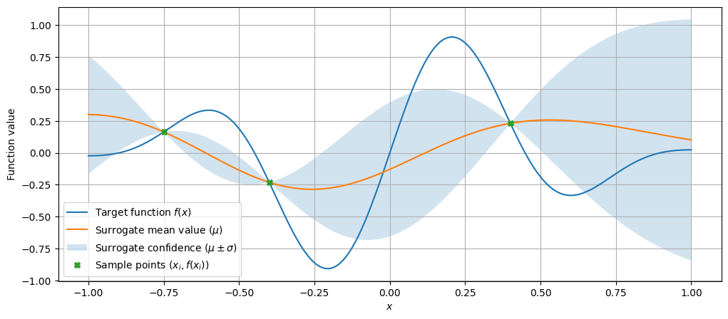

Finally, let’s use the information we gathered to decide which point to try next.

Acquisition functions

We want to use the surrogate estimates to guide the choice of the next evaluation point.

In doing so, we may have conflicting objectives, for instance:

improve the function’s target function: this is, clearly, our bottom line;
improve our knowledge about less explored areas in the domain in order to refine the surrogate and have better chances at finding significant improvements later on.

In general, we we try to capture our criterion into a so called “acquisition function” \(S(x)\) that provides a score for every point \(x\in D\). the value of this score is higher for more desirable points, so that the next chosen point will be the one that maximize \(S\).

We are going to have a look at three easily defined acquisition functions; expected improvement, lower confidence bound, and probability of improvement. Many others are possible, e.g., aiming at the improvement of the process’ entropy, but they lack a closed form and are thus harder to implement.

Expected Improvement

The easiest way to choose our next point is to assume that the mean value returned by the surrogate is a good representation of the function. As we want to define a score to be maximized (while we are looking for the target function’a minimum) let’s define the expected improvement (EI) over the current best as the negative improvement.

The function EI requires the best value found up to now (the lowest \(y\) among all sample points) and the mean value of the surrogate:

def EI_acquisition_function(best: np.float64, mu: np.float64) -> np.float64:
    return best - mu

Let us plot this function across the domain. The highest score highlights the most desirable next evaluation point according to our criterion.

# Find the best target function value among the stored sample points
best = np.min(surrogate.sample_values)
# Compute the acquisition function values for the 400 domain points in X
s_X = [surrogate.evaluate(x) for x in X]
EI_scores = [EI_acquisition_function(best, mu) for mu, _ in s_X]
# Split the plot into two charts; reproduce the surrogate plot
# and the target function on the top for convenience
fig, axes = plt.subplots(2, 1, sharex=True, figsize=(12,8))
axes[0].plot(X, f_X, label='Target function $f(x)$')
surrogate.plot(-1.0, 1.0, axes[0])
# Plot the acquisition function on the second subplot
axes[1].plot(X, EI_scores, label='EI - Expected improvement over current best')
axes[1].set_xlabel('$x$')
axes[1].set_ylabel('Fitness of $x$ as next sample')
axes[1].grid()
axes[1].legend();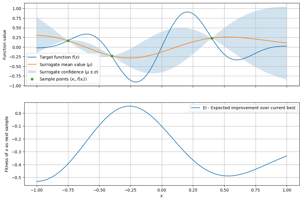

As expected, the EI acquisition function is just an upside-down version of the surrogate mean value.

Lower Confidence Bound

The EI criterion seen above does not take the surrogate’s uncertainty into account. An intuitive way to do this is to look for a point with a chance to have an even better chance of improvement do to its rms estimate. Given the \((\mu,\sigma)\) values returned by the surrogate, we have some probability that the function’s value will be below \(\mu-k\sigma\) (e.g., under normality assumptions we have about 20% probability that \(f(x)<\mu-\sigma\), a 2.5% probability that \(f(x)<\mu-3\sigma\), and so on).

Again, we are looking for a maximizable score. Let us set \(k=1\):

def LCB_acquisition_function(
    best: np.float64,
    mu: np.float64,
    sigma: np.float64
) -> np.float64:
    return best - mu + sigma

This way, the score follows (upside-down) the lowest border of the error band.

# Compute the new acquisition function values for the 400 domain points in X
LCB_scores = [LCB_acquisition_function(best, mu, sigma) for mu, sigma in s_X]
# Reproduce the function and surrogate plot for convenience
fig, axes = plt.subplots(2, 1, sharex=True, figsize=(12,8))
axes[0].plot(X, f_X, label='Target function $f(x)$')
surrogate.plot(-1.0, 1.0, axes[0])
# also plot the previous acquisition function for convenience:
axes[1].plot(X, EI_scores, label='EI - Expected improvement over current best')
axes[1].plot(X, LCB_scores, label='LCB - Lowest confidence bound wrt current best')
axes[1].set_xlabel('$x$')
axes[1].set_ylabel('Fitness of $x$ as next sample')
axes[1].grid()
axes[1].legend();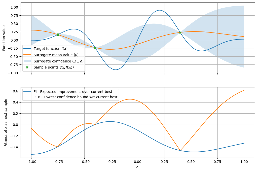

The LCB acquisition function is just an upside-down version of the lower border of the surrogate’s confidence interval.

Probability of Improvement

Let us consider another possible criterion. In this case we are not necessarily interested in the expected size of the improvement, but just in the probability that we will actually find an improvement.

Given the \((\mu(x),\sigma(x))\) values returned by the surrogate for a certain point \(x\in D\), under normality assumptions the probability that we get a value below the current best \(\hat y\) is \(\Pr(f(x)<\hat y) = \Phi(\hat y|\mu=\mu(x), \sigma=\sigma(x))\), where \(\Phi\) is the CDF of the normal distribution with mean \(\mu\) and rms \(\sigma\).

Using the normalized Gaussian distribution, we are looking to maximize \[ \Pr(f(x)>\hat y) = \Phi\left(\frac{\hat y-\mu(x)}{\sigma(x)}\right), \] therefore we define the following acquisition function:

from scipy.stats import norm
def PI_acquisition_function(best: float, mu: float, sigma: float) -> float:
    return norm.cdf((best - mu) / sigma)

Again, let’s plot this latter acquisition function togather with the previous ones:

# Compute the new acquisition function values for the 400 domain points in X
PI_scores = [PI_acquisition_function(best, y, sigma) for y, sigma in s_X]
# Reproduce the surrogate plot for convenience
fig, axes = plt.subplots(2, 1, sharex=True, figsize=(12,8))
axes[0].plot(X, f_X, label='Target function $f(x)$')
surrogate.plot(-1.0, 1.0, axes[0])
# also plot the previous acquisition function for convenience:
axes[1].plot(X, EI_scores, label='EI - Expected improvement over current best')
axes[1].plot(X, LCB_scores, label='LCB - Lowest confidence bound wrt current best')
axes[1].plot(X, PI_scores, label='PI - Probability of improvement wrt current best')
axes[1].set_xlabel('$x$')
axes[1].set_ylabel('Fitness of $x$ as next sample')
axes[1].grid()
axes[1].legend(loc='lower right');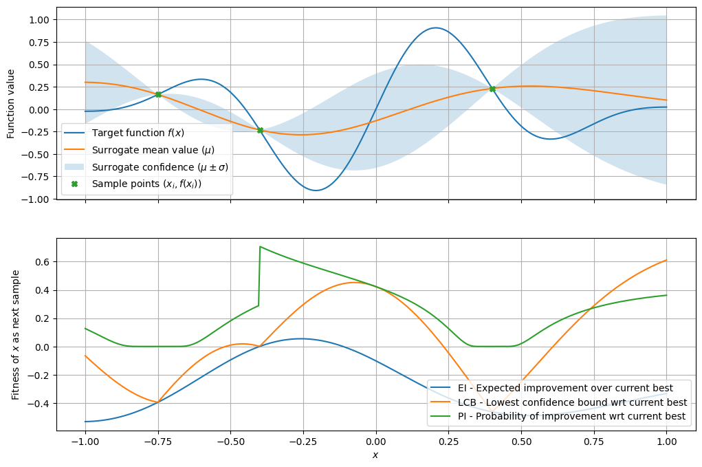

Observe how the PI acquisition function (the green line in the above chart) is sometimes discontinuous around the best sample point. Assume, for instance, that the surrogate is decreasing around the current best (in our case \(x_2=-0.4\)), then any arbitrarily close point to its right has a high probability of improving it.

Bayesian Optimization in action

Let us iterate the optimization for a few steps, and see what happens.

Expected Improvement

For this test we will just initialize the surrogate with the three initial points seen earlier; at each step, we will find the most suitable sample point according to the surrogate and the acquisition function, we will evaluate it with the actual target function and add it to the surrogate.

So, first of all, we initialize the surrogate as before:

surrogate = GaussianProcess(
    dimension=1,
    prior_function=null_prior,
    covariance_function=RBF_covariance
)
for coordinate in np.array([-.75, -.4, .4]):
    x = np.array([coordinate])
    surrogate.add_sample_point(x, f(x))

In order to find the maximum of the acquisition function, we will just perform a grid search across the domain with a large number of sample points, say 10000. There are much more efficient alternatives, but they are outside the focus of this introductory tutorial.

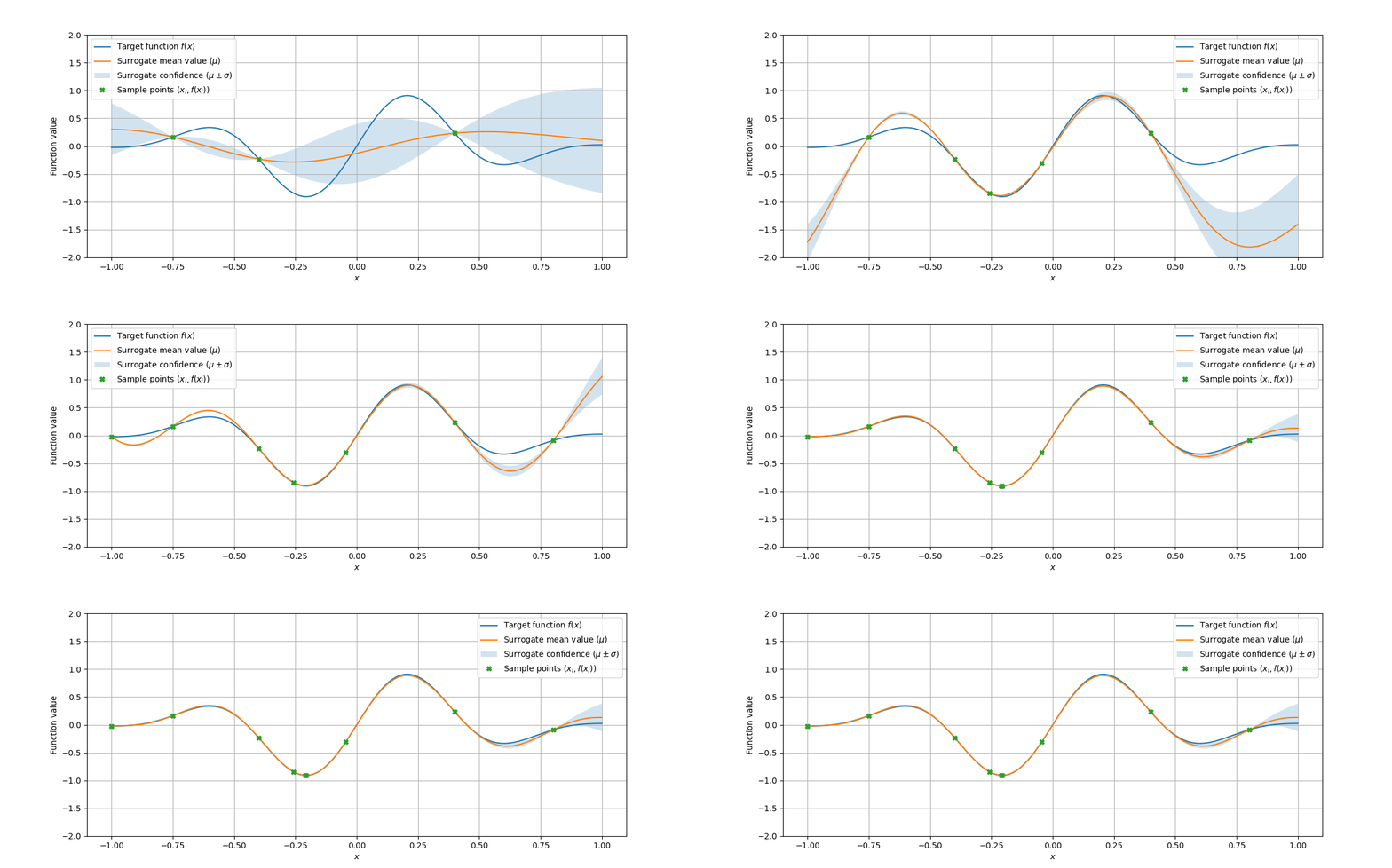
grid_X = np.linspace(-1.0, 1.0, 10000)

Now we are ready to go. We will perform an infinite loop; however, sooner or later the acquisition function will return a point that has already been sampled and the covariance matrix will become singular. At this point, we will break out of the loop.

# Import a few utility functions for animating plots
from IPython.display import display, clear_output
from time import sleep
# we will accumulate a text log of what happens, to be printed below the plot
log = ''
# repeat until something bad happens (see the later try/except block)
while True:
    # Display the target function and the current surrogate state
    clear_output(wait=True)
    plt.close()
    _, axis = plt.subplots(1, 1, figsize=(12,5))
    axis.set_ylim(-2.0, 2.0)
    axis.plot(X, f_X, label='Target function $f(x)$')
    surrogate.plot(-1.0, 1.0, axis)
    axis.set_xlabel('$x$');
    display(plt.gcf())
    # Evaluate the surrogate at all grid points
    s_X = [surrogate.evaluate(x) for x in grid_X]
    # Compute the corresponding scores according to the EI acquisition function
    EI_scores = [EI_acquisition_function(best, mu) for mu, _ in s_X]
    # find the index with the maximum score in the 10000-point grid
    best_index = np.argmax(EI_scores)
    # take the highest-score point (as a numpy array)
    new_sample_point = grid_X[best_index:best_index+1]
    # Finally, evaluate the target function f at the new point
    new_sample_value = f(new_sample_point)
    # Log what has just been done and print it
    log += f'\nbest_index: {best_index}; mu={s_X[best_index][0]}, sigma={s_X[best_index][1]}; x={new_sample_point}, f(x)={new_sample_value}'
    print(log)
    # Add the new sample point (and target function value) to the surrogate;
    # if anything goes wrong, time to wrap up.
    try:
        surrogate.add_sample_point(new_sample_point, new_sample_value)
    except:
        print('Covariance matrix is singular, exiting.')
        break
# forget about the plot, which is already displayed
plt.close()
# print the best point found
best_index = np.argmin(surrogate.sample_values)
best_point = surrogate.sample_points[best_index]
best_value = surrogate.sample_values[best_index]
print(f'Best value {best_value} at {best_point}, after {len(surrogate.sample_points)} target evaluations')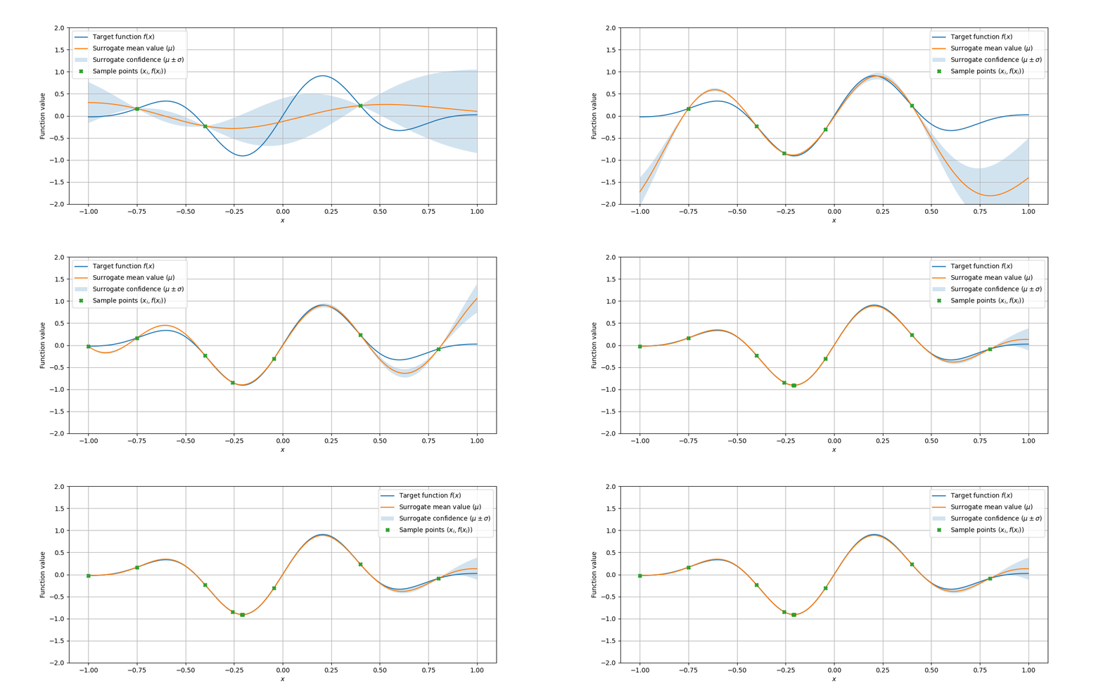


best_index: 3709; mu=-0.2859387318367768, sigma=0.22775715706325295; x=[-0.25812581], f(x)=-0.8434613100663059
best_index: 4777; mu=-1.3528067998513944, sigma=0.15302862273390924; x=[-0.04450445], f(x)=-0.30530225192716415
best_index: 9011; mu=-1.8109821188885507, sigma=0.668576289769467; x=[0.80238024], f(x)=-0.08748090835756739
best_index: 0; mu=-1.870427939484197, sigma=0.3184671808942992; x=[-1.], f(x)=-0.023633397813673053
best_index: 3951; mu=-0.8979055238148641, sigma=0.0026853839529956012; x=[-0.20972097], f(x)=-0.9074490768144003
best_index: 3971; mu=-0.9078545171118101, sigma=1.0101547620395249e-05; x=[-0.20572057], f(x)=-0.9077445088926764
best_index: 3968; mu=-0.9077516642487733, sigma=0.0; x=[-0.20632063], f(x)=-0.9077508804312663
Covariance matrix is singular, exiting.
Best value -0.9077508804312663 at [-0.20632063], after 10 target evaluations

Caveats

What we have seen up to now seems all good: the surrogate nicely approximates the target function, and few target function evaluations are needed to find a near-optimal point.

However, quick self-made code such as that presented above has a very narrow “comfort zone”: just try to replace the acquisition function in the optimization iteration, and you will find interesting and unexpected behavior mainly due to the numerical instability of matrix inversion when many rows and columns are quite similar, due to very close sample points.

The devil is in the details, and having properly working and stable numerical code can be hard. All that we have seen up to now can be easily replaced by few calls to gp_minimize from the scikit-optimize (skopt) Python package, which we suggest for all practical purposes.

Let’s give it a try. First of all, check that the scikit-optimize package is available:

!pip install scikit-optimize

Now, let’s just call the skopt.gp_minimize function on our target function \(f\), on the 1-dimensional interval \([-1,1]\), with EI as acquisition function, 3 initial random sample points and a total of 10 target evaluations:

from skopt import gp_minimize
results = gp_minimize(
    func=f,
    dimensions=[(-1.0, 1.0)],
    acq_func='EI',
    n_random_starts=3,
    n_calls=10,
)

Let’s see the result of the process:

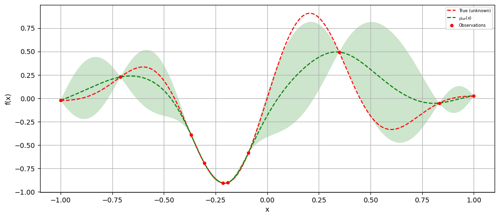
print(f'Best value {results.fun} at {results.x} after {len(results.x_iters)} target evaluations')

Best value -0.905737673494601 at [-0.2152515895620043] after 10 target evaluations

We can see that the best point found is comparable to our one, even slightly better. By default, the surrogate uses a more suitable Matérn kernel in place of our RBF.

We can also plot the resulting process:

from skopt.plots import plot_gaussian_process
_, axis = plt.subplots(1, 1, figsize=(12,5))
plot_gaussian_process(
    results,
    objective=f,
    ax=axis,
    show_legend=True,
    show_title=False,
    show_observations=True,
    show_next_point=False,
    show_acq_func=False
);

In conclusion, it is always quite important to learn by doing things yourself; however, unless you are performing cutting-edge research for which no well-established practices are set, you should always recur to existing code.