Parking a Car with Neural Nets and Local Search

← Greedy Algorithms, part 2

Back to the IO book page

---

This page is a short tutorial on topics covered by the upcoming book Intelligent Optimization - Optimization plus Machine Learning for Reliable Artificial Intelligence by Roberto Battiti, Kevin Tierney and Mauro Brunato.

This tutorial is released under the Creative Commons Attribution-NonCommercial-ShareAlike 4.0 International license (CC BY-NC-SA 4.0)

Prerequisites

To experiment this notebook locally, you must have at least one of the following:

• a working Jupyter notebook server on your computer
• access to a remote notebook server (i.e., Google Colabs);
• a suitable local editor (e.g., Visual Studio Code with the appropriate extension).

To set up all necessary packages in your environment, the following installation command only needs to be run once:

!pip install numpy torch matplotlib ipywidgets

Parking a car

This exercise is about a classical control problem of docking a tractor-trailer truck also used in:

R. Battiti and G. Tecchiolli. “Training neural nets with the reactive tabu search.” IEEE Transactions on Neural Networks, 6(5):1185-1200, 1995.

Here the articulated truck is replaced by a car starting from some random position within an enclosed area and backing up until it docks to a specified point. With some more parameters, similar methods can be applied for docking a satellite in space. But we consider a car because that is closer to the daily experience of all people (we may update the exercise some years from now :).

Car description

The car is described by two fixed dimensional parameters:

• \(d\) is the distance between back and front axles, i.e., the effective length of the car from kinematic purposes;
• \(w\) is the car’s width, only useful for plotting (doesn’t influence the kinematics in our approximation).

The car position is described by three parameters, which will be stored in a torch tensor; in order of entry we have:

• \(x\), \(y\): the \((x,y)\) coordinates of the central point of the back axle (the “license plate” position, if we don’t take the trunk into account). The target docking position is located at \((0,0)\).
• \(\theta\): orientation of the car with respect to the \(x\) axis: the dock is oriented at \(\theta=0\).

These parameters will be subject to some constraints: as soon as the constraints are violated, we deem the car “not viable” anymore:

• \(x\ge0\): the car cannot move past the docking point;
• \(y\ge-3\): we suppose that the area si delimited from below, but we need some leeway to reach the dock;
• \(-90\degree\le\theta_s\le90\degree\): the car must always point left.

The car is backing up at constant speed; the only control variable is therefore

• \(u\): the steering angle of the front wheels.

Although \(u\) is a scalar, we will store it into its own tensor for ease of use.

The Car class

Let’s define a class for the car. First of all, since the car will be controlled by a neural network, let us store all relevant information in pytorch tensors. We will use the torch package; however, as we aren’t going to use gradient-based algorithms, let us disable all gradient and dependency graph internal bookkeeping:

import torch
torch.set_grad_enabled(False);

The Car class has the following members:

• d, w: the dimensional parameters.

• initial_state: the initial values for the positional parameters. We keep them stored so that the car can be reset to its initial position over and over; its components are uniformly chosen in the following intervals: \[\begin{eqnarray*} x&\in&[40, 60]\\ y&\in&[6, 8]\\ \theta&\in&[-6\degree,6\degree]. \end{eqnarray*}\]

• state: the current values for the positional parameters.

• u: the current value of the control variable, also stored as a tensor.

• loss: a velue depending on the car’s state that determines how close it is to the target according to the following weighted tensor norm: \[\begin{equation} \text{loss}(x, y, \theta) = x^2 + \alpha y^2 + \beta\theta^2, \end{equation}\] where \(\alpha=2\) and \(\beta=50\) will be hardcoded and will account for the differences in scale among the state components (\(\theta\) will be expressed in radians).

• viable is a Boolean that tells us if the car can still operate or its parameters are outside the allowed values.

Initially, the methods are the following:

• The constructor receives the dimensional parameters of the car, d and w, it initializes all members.
• reset restores the car to its initial state; it is called by the constructor.
• compute_loss recomputes the loss and viable values at each state change.

class Car:
    d: float
    w: float
    initial_state: torch.Tensor
    state: torch.Tensor
    u: torch.Tensor
    viable: bool
    loss: torch.Tensor

    def __init__(self, d: float = 6, w: float = 4) -> None:
        self.d = d
        self.w = w
        self.initial_state = torch.rand(3) \
            * torch.tensor([20, 2, 12 / 180 * torch.pi]) \
            + torch.tensor([40, 6, -6 / 180 * torch.pi])
        self.state = torch.empty(3)
        self.u = torch.empty(1)
        self.reset()

    def compute_loss(self) -> None:
        self.viable = bool(
            torch.abs(self.state[2]) < 1.5
            and self.state[0] >= 0 and self.state[1] >= -3
        )
        self.loss = self.state[0]**2 + 2*self.state[1]**2 + 50 * self.state[2]**2

    def reset(self) -> None:
        self.state.copy_(self.initial_state)
        self.compute_loss()

Car kinematics

Assuming the state at a given time is \((x, y, \theta)\), for an advancement \(\text dr\) of the motor wheels the following approximate kinematic equations apply: \[ \begin{eqnarray*} \text dA &=& - \text dr\cos u \\ \text dx &=& \text dA\cos\theta \\ \text dy &=& \text dA\sin\theta \\ \text d\theta &=& \arctan\frac{\text dr\sin u}{d} \\ \end{eqnarray*} \]

Let us add a method backup to the class Car that, given the steering angle \(u\) and a small linear movement of the motor wheels \(\text dr\), updates the state of the car, passed as self, and makes it recompute its loss and viability.

Observe that, since the class has already been created, we will initially define the backup method as a separate function accepting a self parameter as first argument:

def backup(self, u: float, dr: float = 1) -> None:
    self.u[0] = u
    x = self.state[0:1]
    y = self.state[1:2]
    theta = self.state[2:3]
    dA = dr * torch.cos(self.u)
    st = torch.sin(theta)
    ct = torch.cos(theta)
    self.state[0:1] -= dA * ct
    self.state[1:2] -= dA * st
    self.state[2:3] -= torch.atan(dr * torch.sin(self.u) / self.d)
    self.compute_loss()

Now we can add the function as a method to class Car:

setattr(Car, backup.__name__, backup)

Display and test

In order to test the kinematics on a simple example, let us create a method that plots the car’s state on a matplotlib.pyplot graph:

import matplotlib.pyplot as plt
def plot(self: Car) -> None:

    # Give local aliases to parameters
    x = self.state[0:1]
    y = self.state[1:2]
    theta = self.state[2:3]
    u = self.u[0]

    # Define the car's shape at resting position, a rectangle docked at (0,0)
    # We define it as a matrix with one point per row because it's easier to
    # understand; however we transpose it because we want column points
    trailer = torch.tensor([
        [0,      -self.w/2],
        [self.d, -self.w/2],
        [self.d,  self.w/2],
        [0,       self.w/2],
        [0,      -self.w/2]
    ]).T

    # We want to rotate the rectangle by theta, let us define the corresponding
    # 2D rotation matrix
    st = torch.sin(theta)
    ct = torch.cos(theta)
    Rt = torch.tensor([
        [ct, -st],
        [st,  ct]
    ])
    # The car rectangle must be rotated (by matrix multiplication),
    # then translated to position (x,y) (as column point)
    transformed_car_rectangle = Rt @ trailer + torch.tensor([[x, y]]).T

    # Define a wheel as a horizontal segment centered in 0
    wheel = torch.tensor([
        [-self.d/10, 0],
        [ self.d/10, 0]
    ]).T
    # Rotate the wheel shape; the steering angle u is defined wrt the car's direction,
    # therefore it must be added to theta:
    su = torch.sin(u + theta)
    cu = torch.cos(u + theta)
    Ru = torch.tensor([
        [cu, -su],
        [su,  cu]
    ])
    rotated_wheel = torch.matmul(Ru, wheel)
    # replicate the wheel twice and anchor it to the appropriate tractor anchor points
    # to avoid cluttering, only the front (steering) wheels are plotted
    left_wheel  = transformed_car_rectangle[:,1:2] + rotated_wheel
    right_wheel = transformed_car_rectangle[:,2:3] + rotated_wheel
    # plot all polygons
    plt.plot(transformed_car_rectangle[0], transformed_car_rectangle[1], 'r')
    plt.plot(left_wheel[0], left_wheel[1], 'b', linewidth=3)
    plt.plot(right_wheel[0], right_wheel[1], 'b', linewidth=3)

# Add the function to the Truck class as a method:
setattr(Car, plot.__name__, plot)

Testing the plotting function

Let us generate a random car and plot it in a conveniently large field:

plt.close()
plt.xlim(0, 80)
plt.ylim(-10, 30)
plt.grid()
car = Car()
car.plot()
plt.gca().set_aspect('equal')
plt.show()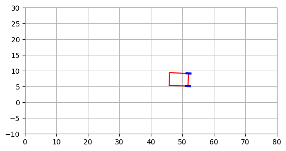

Testing the kinematics

Now we want to plot the evolution of the car backing up for a small number of steps, with a random steering angle at each step, and plot it at every step:

car = Car()
plt.xlim(0, 80)
plt.ylim(-10, 30)
car.plot()
while car.viable:
    car.backup(u=(torch.rand(1)-.5), dr=1)
    car.plot()
plt.grid()
plt.gca().set_aspect('equal')
plt.show()
plt.close()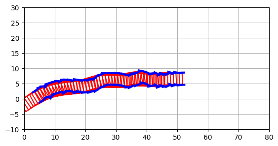

Animating the car

Finally, let us “animate” the car. The following function simulate_truck accepts two functions that must be provided by the caller:

• steering_angle is the function that “drives” the car: it accepts the car’s object and must return the steering angle to use;
• caption_text accepts the car’s object and provides a title for the current frame: it can be used to show the current state.

The function uses specific IPython functions to animate the output. It takes the truck as first parameter so that it can be incorporated as method.

from typing import Optional
from collections.abc import Callable
from IPython.display import display, clear_output
from time import sleep
def animate(
    self: Car,
    steering_angle: Callable[[Car], float],
    caption_text: Callable[[Car], str]
) -> None:
    self.reset()
    while self.viable:
        clear_output(wait=True)
        plt.close()
        plt.xlim(0, 80)
        plt.ylim(-10, 30)
        plt.grid()
        plt.title(caption_text(self))
        plt.plot([0], [0], 'Dg', markersize=10)
        self.plot()
        plt.gca().set_aspect('equal')
        display(plt.gcf())
        self.backup(steering_angle(self), 1)
        sleep(.01)
    clear_output(wait=True)
    plt.gca().set_aspect('equal')
    display(plt.gcf())
    plt.close()
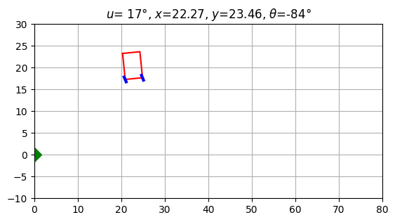
setattr(Car, animate.__name__, animate)

Let us test this function by simulating a run with null steering; see how caption_text is used to display the car’s coordinates in real time.

Car().animate(
    steering_angle=lambda _: 0.0,
    caption_text= lambda t:
        f'$x$={t.state[0]:.2f}, $y$={t.state[1]:.2f}, $\\theta$={t.state[2]:.3f}'
)

Bonus section: try it!

Nota bene — this section only works if you are currently running this notebook; otherwise, you’ll only see static images.

If you run this notebook locally, you can try to actually drive the car.

For this demo, let us create two widgets to control the simulation:

• steering_angle_controller is a slider that sets the steering angle \(u\); for clarity we will set the angle in degrees, when needed we will convert it into radians;
• execution_controller is a checkbox that, when unchecked, halts the simulation.

The values of the two widgets will be used by later code.

import ipywidgets as widgets
steering_angle_controller = widgets.FloatSlider(
    value=0.0, min = -60.0, max = 60.0, step=1
)
execution_controller = widgets.Checkbox(
    value=True, description='Uncheck to stop running', indent=False
)
display(steering_angle_controller, execution_controller)

Now, let us repeatedly call the simulation function. The steering_angle function just translates the float value of the steering_angle_controller slider into radians and forwards it to the function; caption_text reports useful information.

You can try to dynamically change the steering angle while running, however your results may vary…

while execution_controller.value:
    sleep(1)
    Car().animate(
        steering_angle = lambda _: steering_angle_controller.value/180*torch.pi,
        caption_text = lambda car:
            f'$u$={steering_angle_controller.value:3.0f}°, $x$={car.state[0]:5.2f}, $y$={car.state[1]:5.2f}, $\\theta$={car.state[2]/torch.pi*180:3.0f}°'
    )

Learning to park

Let’s now define a driver for our car. Our driver will be a neural network with as many inputs as state variables (in our case 3: \(x\), \(y\) and \(\theta\)) and one output controlling the steering angle \(u\).

It is easy to see that a feedforward network is enough for our purposes: the driver has no reason to have an internal state: the optimal steering angle at a certain moment only depends on the immediate state of the car, regardless of its past history.

We will provide a small but significant hidden layer (32 nodes) with a ReLU activation function. The output will pass through a hyperbolic tangent so that it is symmetrically constrained between \(-1/2\) and \(1/2\):

driver = torch.nn.Sequential(
    torch.nn.Linear(3, 32),
    torch.nn.ReLU(),
    torch.nn.Linear(32, 1),
    torch.nn.Tanh()
)

We can immediately test our driver by invoking it in the steering_angle argument of the animate method created above.

Don’t get your hopes up, though: an untrained network cannot be expected to do any good:

Car().animate(
    steering_angle = lambda car: driver(car.state),
    caption_text = lambda car:
        f'$u$={car.u[0]/torch.pi*180:4.2f}°, $x$={car.state[0]:5.2f}, $y$={car.state[1]:5.2f}, $\\theta$={car.state[2]/torch.pi*180:3.0f}°'
)

Let’s write a utility function that runs a large number of cars (while viable) and returns the average final loss.

The function requires two arguments:

• driver: the driver neural net
• cars: a list of cars on which the driver is tested

The function returns the average loss.

def test_drive_loss(driver: torch.nn.Module, cars: list[Car]) -> float:
    cumulated_loss = 0.0
    for car in cars:
        car.reset()
        while car.viable and car.loss > 1:
            car.backup(driver(car.state))
        cumulated_loss += car.loss.item()
    return cumulated_loss / len(cars)

Let’s test the untrained driver on a set of 100 cars:

loss = test_drive_loss(
    driver,
    [Car() for _ in range(100)]
)
print(f'Test drive average loss is {loss:.2f}')

Test drive average loss is 2274.80

Training the driver

The driver network is designed to map the state \((x,y,\theta)\) of the car to the immediate action \(u\). The way we want to use it is to place the car in the initial position, provide its state to the driver, get the steering angle \(u\) and apply it, back up a little, repeat as long as the car is viable (as in the test drive above).

This way, however, we won’t know if a specific driver response was adequate or not immediately after it was provided: only at the end, when the car becomes “not viable”, we will be able to know if our target has been reached.

Classically, a neural network is trained by computing a differentiable error function and “backpropagating” the error. The way we apply the driver to the problem, however, doesn’t yield a clearly differentiable function, so let us try to minimize the driver’s error by local search applied to the driver’s parameters.

To do so, we will need to represent the fitness of our driver as a function \(f(\boldsymbol x)\) where \(\boldsymbol x\) is a flat numpy array, while the function’s value represents the average badness of the driver throughout various test drives.

In detail, to evaluate \(f(\boldsymbol x)\):

• interpret the input array \(\boldsymbol x\) as the sequence of all model weights (copy \(\boldsymbol x\) into the parameters structure of the driver model;
• simulate a sequence of test drives recording the final loss function of each drive;
• return the average loss as a measure of the driver’s badness.

Since the torch model’s parameter structure is not flat (a single array), but it is a dictionary of tensors, we need a few utility functions. The first get_n_parameters, returns the number of parameters of a torch model:

def get_n_parameters(model: torch.nn.Module) -> int:
    n = 0
    # Scan the parameters dictionary
    for component_parameters in model.state_dict().values():
        # every item should be a tensor (if None, then something is wrong)
        assert type(component_parameters) == torch.Tensor
        # Add the number of parameters from the current layer
        n += component_parameters.shape.numel()
    # Return the cumulated sum
    return n

The second utility function we need is used to take the parameters from a (flat) numpy array and copy them into the appropriate parameter tensors of the model:

import numpy as np
def set_parameters_from_numpy_array(
    model: torch.nn.Module,
    parameters: np.ndarray
) -> None:
    # First index in the numpy array not yet used
    n = 0
    # Scan all parameter tensors in the model
    for component_parameters in model.state_dict().values():
        # every item should be a tensor
        assert type(component_parameters) == torch.Tensor
        # get the shape of the tensor and the corresponding number of entries
        size = component_parameters.shape
        l = size.numel()
        # intrepret the section [n:n+l] of the numpy vector as an array
        # with the same shape of the tensor and copy it
        component_parameters.copy_(torch.tensor(parameters[n:n+l]).view(size))
        # advance by l
        n += l

We are now ready to define the function that we want to be minimized.

The function acts as a wrapper for the test_drive_loss function defined before, but it requires as only argument the array of neural network parameters to be optimized: it will update the network parameters using the utility function set_parameters_from_numpy_array, then it returns the corresponding test drive loss:

training_cars = [Car() for _ in range(100)]
def training_loss(driver_parameters: np.ndarray) -> float:
    global driver, training_cars
    set_parameters_from_numpy_array(driver, driver_parameters)
    return test_drive_loss(driver, training_cars)

The optimization algorithm that we are going to use is the Reactive Affine Shaker (RAS) algorithm, from our CoRSO package, described in:

R. Battiti and G. Tecchiolli. Learning with first, second, and no derivatives: a case study in high energy physics. Neurocomputing, 6:181–206, 1994.

The algorithm allows the user to define a callback that is invoked every time there is an improvement in the target value. The callback must accept three arguments:

• the array achieving the improved value
• the improved value
• the number of evaluations performed since the algorithm start

We will use the function to test the parameters on a separate validation set of cars and, if the validation results confirm the improvement, we will store the new parameter set in a global array to be used later.

validation_cars = [Car() for _ in range(100)]

# Initial validation values
best_validation_parameters: Optional[torch.Tensor] = None
best_validation_loss = np.inf

def improvement_callback(
    driver_parameters: np.ndarray,
    training_loss: float,
    evaluations: int
) -> bool:
    global driver, validation_cars, best_validation_parameters, best_validation_loss
    set_parameters_from_numpy_array(driver, driver_parameters)
    validation_loss = test_drive_loss(driver, validation_cars)
    print(f'New training minimum found: {training_loss:8.3f} @ eval {evaluations:5d}; validation: {validation_loss:8.3f}')
    if validation_loss < best_validation_loss:
        best_validation_parameters = driver_parameters.copy()
        best_validation_loss = validation_loss
    return True

Now we have all elements to run the optimization. As a final touch, to ensure repeatability, let us set a fixed random seed on all random libraries that will be used in this tutorial: torch, numpy and Python’s baseline random package.

Feel free to change the random seed to check the effect of different local minima on the overll car behavior.

seed = 7635

import random
random.seed(seed)
np.random.seed(seed)
torch.manual_seed(seed);

We will use the ras_solver function from the CoRSO package; the function accepts the following arguments:

• the function to be optimized, in our case training_loss define above, accepting a numpy array and returning a float;
• the dimensionality, i.e. the number of parameters to be optimized;
• the number of target function evaluations before halting;
• the optional improvement callback (as defined above).

Usually, an array of parameter lower bounds and another for upper bounds would be required, but they default to reasonable values for a neurral network (the interval \([-1,1]\)), so we needn’t specify them.

Thanks to the callback, a report line will be printed every time a better solution is found. At the end, the array best_validation_parameters contains the best solution found on the validation list of cars.

from CoRSO.solver import ras_solver
dimensionality = get_n_parameters(driver)
best_x, best_y = ras_solver(
    training_loss,
    dimensionality,
    max_evaluations = 1000,
    improvement_callback=improvement_callback
)

New training minimum found: 2216.608 @ eval     1; validation: 2331.387
New training minimum found:  251.651 @ eval     3; validation:  156.973
New training minimum found:   12.028 @ eval     8; validation:   11.817
New training minimum found:    9.167 @ eval    17; validation:    7.577
New training minimum found:    4.777 @ eval    21; validation:    5.165
New training minimum found:    4.468 @ eval    50; validation:    4.198
New training minimum found:    3.361 @ eval   121; validation:    3.468
New training minimum found:    2.699 @ eval   136; validation:    2.755
New training minimum found:    0.928 @ eval   156; validation:    0.970
New training minimum found:    0.862 @ eval   168; validation:    0.870
New training minimum found:    0.353 @ eval   174; validation:    0.365
New training minimum found:    0.301 @ eval   184; validation:    0.275
New training minimum found:    0.255 @ eval   521; validation:    0.314

Testing the best solution found

Let’s now restore the best validation parameters onto the driver:

set_parameters_from_numpy_array(driver, best_validation_parameters)

We are ready to animate the first 10 validation cars and see if their trajectory is reasonable or not:

for car in validation_cars[:10]:
    car.animate(
        steering_angle = lambda car: driver(car.state),
        caption_text = lambda car:
            f'$u$={car.u[0]/torch.pi*180:6.2f}°, $x$={car.state[0]:5.2f}, $y$={car.state[1]:5.2f}, $\\theta$={car.state[2]/torch.pi*180:3.0f}°'
    )

The solution depends on the actual (local) optimum found in the parameter space. You may want to try with different random seeds.

In some cases, the car moves smoothly; in other cases, the driver oscillates as if overcompensating its previous errors (which can be a very human behaviour :). Indeed, our only criterion is the final result: as long as the car docks correctly on the origin, its previous behavior doesn’t count.

A useful exercise is to modify the objective function so that smoother trajectories are preferred, we will do that in a future exercise.