!pip install numpy matplotlibReactive Affine Shaker
This is a tutorial on topics covered by the Intelligent Optimization - Optimization meets Machine Learning by Roberto Battiti, Mauro Brunato and Kevin Tierney, released under the Creative Commons Attribution-NonCommercial-ShareAlike 4.0 International license (CC BY-NC-SA 4.0).
Prerequisites
In order to be able to experiment this notebook locally, you must have at least one of the following:
- a working Jupyter notebook server on your computer
- access to a remote notebook server (i.e., Google Colabs);
- a suitable local editor (e.g., Visual Studio Code with the appropriate extension).
To set up all necessary packages in your environment, the following installation command only needs to be run once:
Optimizing a continuous function
We implement a basic Python version of the Reactive Affine Shaker (RAS) heuristic described in the book and in the original papers [1][2][3][4][5][6].
We optimize (in this case, minimize) a continuous function of real variables, \[\begin{eqnarray*} f: D &\to& \mathbb{R}\\ x &\mapsto& f(x) \end{eqnarray*}\] where \(D\) is usually a compact subset of \(\mathbb{R}^d\); we refer to \(d\) as the dimensionality of the problem.
Our purpose is to find the function’s global minimum \[ x^* = \mathop{\text{argmin}}\limits_{x\in D}f(x). \]
The Rosenbrock function
Several benchmark functions have been historically proposed to test continuous minimization heuristics. One of them is the Rosenbrock function. Let \(\boldsymbol{x}=(x_1,x_2,\dots,x_d)\in D=[-5,10]^d\). Then \[ f(\boldsymbol{x}) = \sum_{i=1}^{d-1}\bigl[100(x_{i+1}-x_i^2)^2+(1-x_i)^2\bigr]. \] It is possible to show that the function’s global minimum is attained at \((x_1,\dots,x_d)=(1,\dots,1)\).
Let us define it with the help of numpy. In order to better illustrate things, we work in \(d=2\) dimensions; however, most of the code is kept general.
Also note that, to keep boilerplate code to a minimum, we use global variables and we don’t make use of classes.
First of all, let’s define the dimensionality and the domain \(D\) in terms of a lower_bound and an upper_bound array.
import numpy as np

dimension = 2
lower_bound = np.full((dimension,), -5.0)
upper_bound = np.full((dimension,), 10.0)
The function itself, called rosenbrock, accepts a Numpy array as input and provides a float-like value as output.
def rosenbrock(x: np.ndarray) -> float:
    xshort = x[:-1] # all elements but the last
    xshift = x[1:]  # all elements but the first, to easily access x[i+1] via index i
    return np.sum(100.0 * (xshift - xshort**2)**2 + (1.0 - xshort)**2)
Let’s now take a look at the function’s chart, of course under the assumption that the dimension is 2.
First, let’s define a set of 400 points both along the \(x\) and the \(y\) axis:
x_array = np.linspace(lower_bound[0], upper_bound[0], 400)
y_array = np.linspace(lower_bound[1], upper_bound[1], 400)
Create the two mesh grids required by Matplotlib for a contour plot. The first, x_mesh, contains an array of arrays of all \(x\) coordinates of the \(400\times400\) grid points; y_mesh contains the corresponding \(y\) coordinates:
x_mesh, y_mesh = np.meshgrid(x_array, y_array)For every point \(\boldsymbol{x}=(x,y)\) in the mesh we want the corresponding \(z=\texttt{rosenbrock}(\boldsymbol{x})\) value; for this, we first combine the two meshes into a three-index temsor whose last dimension spans the two coordinates, then we compute the function along the first two dimensions.
Note that the function has a very wide range; in order to be able to visualize the neighborhood of the local minimum, we take the logarithm of the result:
xy_mesh = np.stack([x_mesh, y_mesh], -1)
z_mesh = np.array([[np.log(rosenbrock(xy)) for xy in row] for row in xy_mesh])
We are finally ready to plot the function’s contour.
import matplotlib.pyplot as plt

# make a square plot because the domain is square
plt.gca().set_box_aspect(1)
# plot the function's contour at 15 equally spaced levels
plt.contour(x_mesh, y_mesh, z_mesh, levels=15)
# Mark the global minimum (1,1) with a red cross
plt.plot(1.0, 1.0, 'xr')
# Add a grid for reference
plt.grid();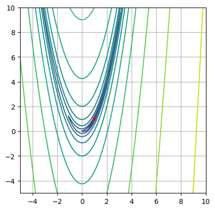
The function is characterized by steep descending walls leading to a narrow parabolic valley, with an almost flat bottom where the minimum is located. The shape of the valley is the source of the nickname “Banana function”.
Defining the search heuristic
RAS is still a local search heuristic. This means that we maintain a “current best” solution and perturb it with (relatively) small variations.
The initial position
Let us set a convenient random number generator seed so that we can repeat the experiment if needed:
np.random.seed(100)Next, we define two global variables to store the current best position, initially a uniformly selected random point in the domain, and the corresponding function value:
current_position = np.random.uniform(lower_bound, upper_bound)
current_value = rosenbrock(current_position)
The heuristic parameters
The RAS heuristic is based on three independent parameters:
initial_size(\(0<\eta<1\) in the literature): the initial half-size of the search box around the current point expressed as a fraction of the domain size along the same dimension;contraction_factor(\(0<\rho_{\text{con}}<1\)): the amount of contraction the search box undergoes after a failed perturbation attempt;dilation_factor(\(\rho_{\text{dil}}>1\)): the amount of dilation to apply to the search box along the direction of a successful perturbation attempt.
initial_size = .1
contraction_factor = .9
dilation_factor = 1.0 / contraction_factor
The search box
As we know, the search box is represented by \(d\) “basis” vectors \(\boldsymbol{b}_1,\dots,\boldsymbol{b}_d\in\mathbb{R}^d\). Given that we have \(d\) vectors in a \(d\)-dimensional space, we can compactly represent them as rows in a \(d\times d\) real-valued matrix. This matrix representation will be useful because it allows us to update all vectors with one statement.
As we want to initialize them as parallel to the coordinate axes, the matrix is initially the identity, rescaled according to the domain sizes (difference between upper and lower bound along the different dimensions) and by the initial_size parameter:
current_basis = initial_size * (upper_bound - lower_bound) * np.identity(dimension)
print(current_basis)
[[1.5 0. ]
[0. 1.5]]Displaying the search box
Let us define a function that displays a box with the two vectors in the \(d=2\) case. We use that function several times in the next part.
The function accepts three arguments:
- the
axis(subplot) on which the box must be plotted (if none, then the whole figure is used); - the
positionof the current point; - the
basisvectors of the box in the form of a square matrix.
def display_box(axis, position, basis):
    # if no axis given, then use the whole plot
    if axis is None:
        axis = plt.gca()
    # make a square plot
    axis.set_box_aspect(1)
    # use the same scale on both coordinate axes
    axis.set_aspect('equal')
    # plot the position as a red circle
    axis.plot(position[0], position[1], 'or')
    # draw black arrows corresponding to the vectors
    # contained in the two basis matrix rows
    axis.annotate('', xytext=position, xy=position+basis[0],
                  arrowprops=dict(arrowstyle="->"))
    axis.annotate('', xytext=position, xy=position+basis[1],
                  arrowprops=dict(arrowstyle="->"))
    # draw a green box delimiting the area defined by the basis vectors
    box = np.array([
        position-basis[0]-basis[1],
        position-basis[0]+basis[1],
        position+basis[0]+basis[1],
        position+basis[0]-basis[1],
        position-basis[0]-basis[1]
    ])
    axis.plot(box[:,0], box[:,1], 'g')
Let’s test the function on the current position and basis:
display_box(None, current_position, current_basis)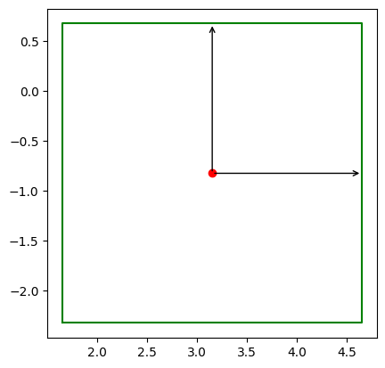
To better examine the behavior of the heuristic, let us define a list containing the past history of the optimization. Every entry in the list corresponds to a step in the algorithm and contains the following information:
- the current position at that step
- the corresponding function falue
- the corresponding base vector matrix for the search box
trajectory = [(current_position, current_value, current_basis)]Based on this, let us define a function that plots the whole search trajectory and superimposes it on the function’s contour plot. The function improves the plotting code that we used at the beginning of this tutorial and will receive two optional arguments:
- the
axis(subplot) on which the trajectory can be plotted; - the
stepup to which we want to plot the trajectory (so that we can display the status at any arbitrary past step).
def draw_history(axis=None, step=None):
    # this function refers to a lot of globals
    global x_mesh, y_mesh, z_mesh, trajectory
    # if no axis is given, use the current one
    if axis is None:
        axis = plt.gca()
    # we want a square plot
    axis.set_box_aspect(1)
    # coordinates must have the same scale
    axis.set_aspect('equal')
    # if step is given, just use the initial sechion of the trajectory
    visible_trajectory = trajectory if step is None else trajectory[:step+1]
    # current position and basis are given by the last visible step
    position, _, basis = visible_trajectory[-1]
    # draw the contour plot
    axis.contour(x_mesh, y_mesh, z_mesh, levels=15)
    # mark the global optimum with a red cross
    axis.plot(1.0, 1.0, 'xr')
    # trace the trajectory with a red line
    axis.plot([x[0] for x,_,_ in visible_trajectory],
              [x[1] for x,_,_ in visible_trajectory], 'r')
    # draw the search box at the given step by using the previously defined function
    display_box(axis, position, basis)
    # add a grid
    axis.grid()
Let’s test the function. As the trajectory contains but one item, only the current position and box are displayed (no past history yet):
draw_history()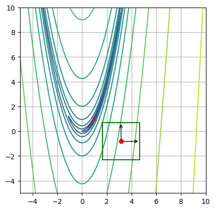
The search step
Before we write a function to perform a repeated search iteration, let us examine all steps.
First of all, we generate a \(d\)-dimensional displacement delta in the search box by computing a uniform random linear combination of the basis vectors, each with a coefficient in \([-1,1]\). In the initial step, this provides a random vector with components in \([-1.5,1.5]\):
delta = np.random.uniform(-1, 1, dimension) @ current_basis
print(delta)
[-0.22644723 1.0343284 ]Next, we add the displacement vector to the current position and we check if the function value has been reduced. If so, we report success. If not, we make another attempt by subtracting the same displacement. The rationale is that if the function is smooth enough inside the search box it may have a near-linear behavior.
for shot in [1, -1]: # either add or subtract
    # apply the displacement in the required direction
    new_tentative_position = current_position + shot * delta
    # compute the corresponding function value
    new_tentative_value = rosenbrock(new_tentative_position)
    # if the value improved, then success and terminate the loop
    success = new_tentative_value < current_value
    if success:
        break
In this case, we can see that one of the two displacements has succeeded (success is true):
print(current_value, new_tentative_value, success)11568.892368896679 6965.2257727374545 TrueNow, based on the success (or lack thereof) of our perturbation, we decide what to do.
- if the step succeeded, we update the current position and value to the new ones; moreover, we choose the dilation factor for the subsequent box modification, so that exploration along the direction of the successful displacement is encouraged;
- if it didn’t succeed, then we don’t move the current position and choose the contraction factor to contract the box along the same direction.
if success:
    current_position = new_tentative_position
    current_value = new_tentative_value
    factor = dilation_factor
else:
    factor = contraction_factor
Finally, we resize the basis vectors along the displacement \(\boldsymbol\delta\) (delta) based on the chosen value of \(\rho\) (factor, either dilation or contraction).
Remember that the resizing matrix, that we can directly apply to the basis vectors, is defined as \[ A = \mathbb1_d + (\rho-1)\frac{\boldsymbol\delta\cdot\boldsymbol\delta^T}{\|\boldsymbol\delta\|^2}, \] where \(\mathbb1_d\) is the \(d\times d\) identity matrix.
# Compute the update matrix
A = np.identity(dimension) \
    + (factor-1) \
        * (delta.reshape(dimension,1) @ delta.reshape(1,dimension)) \
        / sum(delta**2)
# Apply the update matrix to the basis vectors creating a new copy
current_basis = A @ current_basis
Let’s append the new point and basis to the trajectory list:
trajectory.append((current_position, current_value, current_basis))We can now display the trajectory vith our plotting function to see our first step and the modified box (notice that the basis vectors and the box sides are slightly askew now):
draw_history()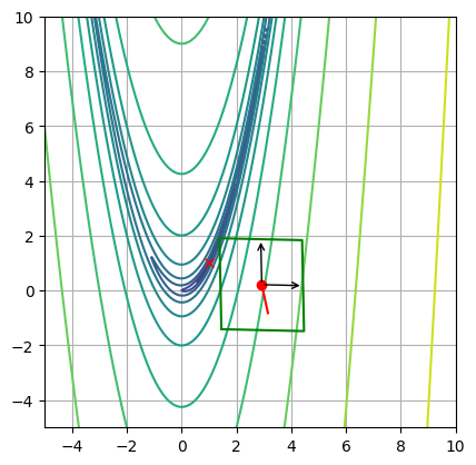
Let us collect all previous code into a function, so that we can apply it at will:
def step():
    global dimension, current_basis, current_position, current_value
    global contraction_factor, dilation_factor, trajectory
    delta = np.random.uniform(-1, 1, dimension) @ current_basis
    for shot in [1, -1]:
        new_tentative_position = current_position + shot * delta
        new_tentative_value = rosenbrock(new_tentative_position)
        success = new_tentative_value < current_value
        if success:
            break
    if success:
        current_position = new_tentative_position
        current_value = new_tentative_value
        factor = dilation_factor
    else:
        factor = contraction_factor
    A = np.identity(dimension) \
        + (factor-1) \
            * (delta.reshape(dimension,1) @ delta.reshape(1,dimension)) \
            / sum(delta**2)
    current_basis = A @ current_basis
    trajectory.append((current_position, current_value, current_basis))
Apply a new step and see the history.
step()
print(current_value)983.5731966049806draw_history()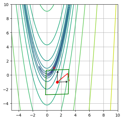
Again, for a few more steps:
for i in range(20):
    step()
draw_history()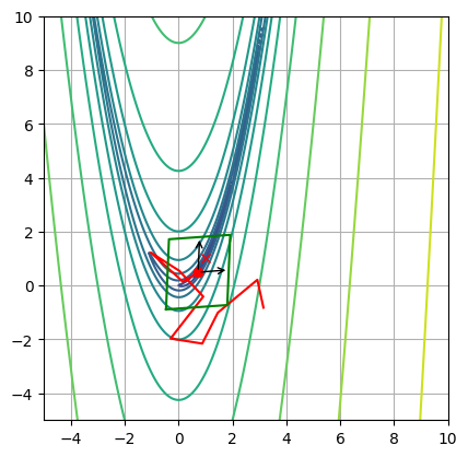
Now let’s apply many more steps and let the search evolve:
for i in range(400):
    step()
Trajectory analysis
At this point, we may want to see the full search trajectory paired with the evolution of the current minimum at each step (the “best so far” value). Let’s also get an idea of the evolution of the search box size by plotting the basis matrix Frobenius norm.
Note that the Frobenius norm isn’t necessarily the most indicative way of measuring our search box (the relative alignment of the basis vectors is also important), but we want to keep things simple.
# Prepare two subplots
figure, (axis1, axis2) = plt.subplots(ncols=2)
# Set the overall size
figure.set_size_inches(10,5)
# Draw the search trajectory on the first subplot
draw_history(axis1)
# make the seconf plot rectangular
axis2.set_box_aspect(3/4)
# make it semi-logarithmic (the scale changes a lot)
axis2.set_yscale('log')
# Plot the best so far
axis2.plot([value for _,value,_ in trajectory], label='best so far')
# Plot the basis matrix norms
axis2.plot([np.linalg.norm(basis) for _,_,basis in trajectory[1:]], label='box size')
# Add a grid, a legend and a horizontal axis label
axis2.grid()
axis2.legend()
axis2.set_xlabel('Step');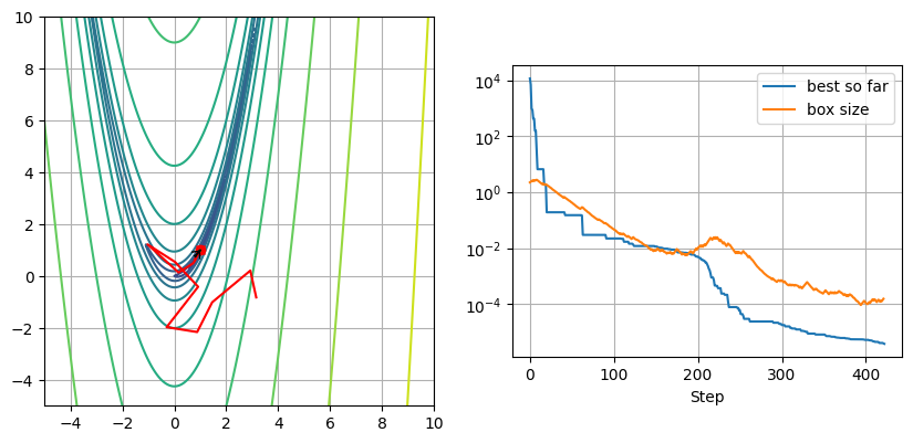
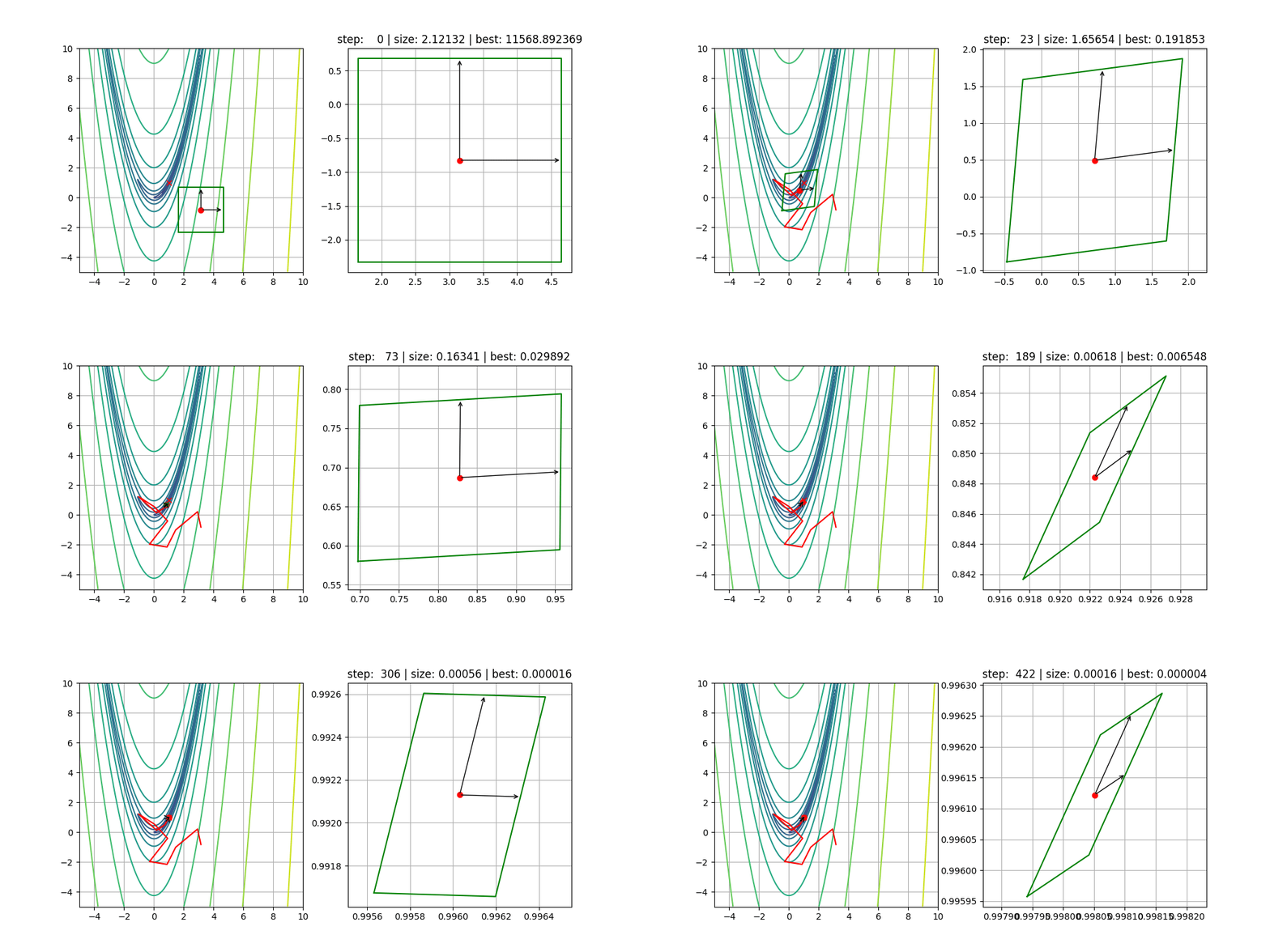
The trajectory shown in the left plot shows that with few large downhill steps the heuristic easily finds the valley (by basically applying random displacements, since every direction leads to some improvement).
After that, the function value is steadily improved by much smaller steps, but the overall box size tends to decrease due to many failures. This can be expected: as the valley narrows down, if the generated displacement isn’t aligned with it both evaluations fail because will climb up on the two sides.
Also note that after iteration 200 the box size temporarily grows up, indicating a sequence of successes and corresponding to a steep improvement in the function value, probably due to the successful alignment of the search box to the valley. This is the part in which RAS is probably most effective.
Selected steps
Let us write a utility function that displays the trajectory up to a given step (by invoking draw_history) and an enlarged plot of the search box to examine its shape.
def show_partial_history(step):
    global trajectory
    # create two subplots
    figure, (axis1, axis2) = plt.subplots(ncols=2)
    #set the figure size
    figure.set_size_inches(10,5)
    # draw the usual trajectory in the first subplot
    draw_history(axis1, step)
    # take the position and basis matrix at the given step
    position, _, basis = trajectory[step]
    # show the box on the second plot
    display_box(axis2, position, basis)
    axis2.grid()
We can now see the status of the box after 10 steps:
show_partial_history(10)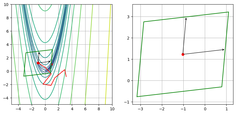
The heuristic has complete the simple task of falling down to the valley.
At step 20:
show_partial_history(20)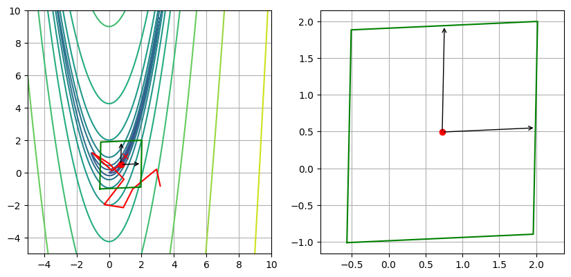
The trajectory has begun to follow the valley and proceeds down to step 100:
show_partial_history(100)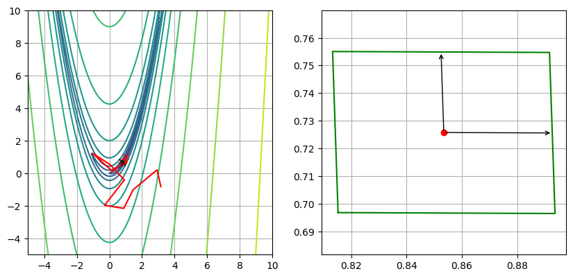
Here we can see that the search region has remained almost rectangular but has drastically shrunk: the valley isn’t so narrow to enforce a direction yet, but failures keep happening.
The following picture represents the status at the end of the steep descent of steps 200-250:
show_partial_history(250)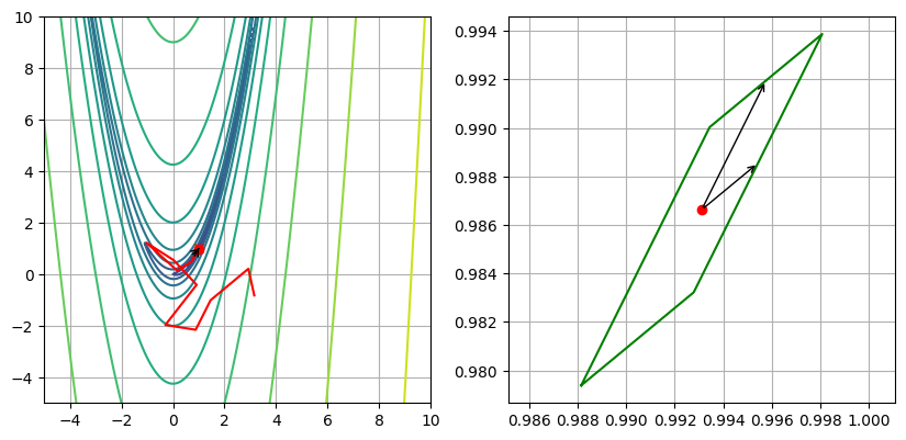
Here the search box is very small and very elongated along the valley’s direction. This is the case until the very last iteration:
show_partial_history(len(trajectory)-1)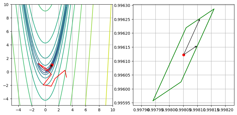
The full search
Let us loop across all steps and use the animation features to have a look at the whole evolution.
The actual box size is hard to grasp, since it is normalized in the second plot, but we can focus on its shape.
from IPython.display import display, clear_output
from time import sleep

for step in range(len(trajectory)):
    clear_output(wait=True)
    plt.close()
    show_partial_history(step)
    plt.title(f'step: {step:4} | size: {np.linalg.norm(trajectory[step][2]):7.5f} | best: {trajectory[step][1]:8.6f}')
    display(plt.gcf())
    sleep(.001)
plt.close()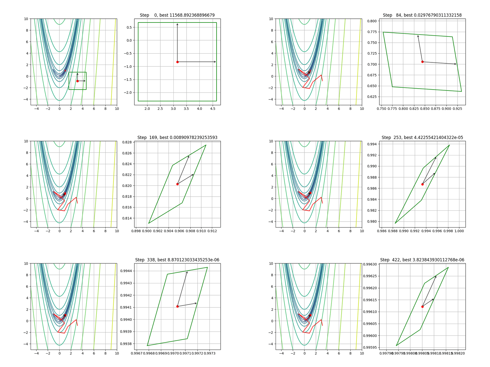
Conclusion
The code developed here is for instructional purposes only. An up-to-date and production-ready C++ implementation of the RAS heuristic (and of its close relative, the Inertial Shaker) is available as a Python package in the Pypi repository, free for use for non-commercial purposes. It includes: - encapsulation, - checks about divisions by very small numbers and other numerical instabilities, - checks about the current point leaving the function’s domain with a strategy to bring it back inside, - optimized array and matrix operations, - faster CPU times due to the C++ compiled code.
References
- R. Battiti and G. Tecchiolli. Learning with first, second, and no derivatives: a case study in high energy physics.
Neurocomputing, 6:181-206, 1994.
| PDF | - M. Brunato and R. Battiti. The Reactive Affine Shaker: a Building Block for Minimizing Functions of Continuous Variables.
DIT Technical Report DIT-06-012, University of Trento, March 2006.
| Catalog page | PDF | - M. Brunato, R. Battiti, and S. Pasupuleti. A Memory-Based RASH Optimizer.
DIT Technical Report DIT-06-023, University of Trento, March 2006.
| Catalog page | PDF | - M. Brunato, R. Battiti, and S. Pasupuleti. A memory-based rash optimizer.
In: AAAI-06 Workshop on Heuristic Search, Memory Based Heuristics and Their applications. Boston, Mass., USA, July 17, 2006.
| PDF | - M. Brunato and R. Battiti. RASH: A self-adaptive random search method.
In: C. Cotta, M. Sevaux, and K. Sörensen, eds. Adaptive and Multilevel Meta-heuristics. Studies in Computational Intelligence 136:95-117, Springer, 2008.
ISBN: 978-3-540-79437-0, DOI: https://doi.org/10.1007/978-3-540-79438-7_5
| Editor page | - R. Battiti and M. Brunato. Pushing the Limits of the Reactive Affine Shaker Algorithm to Higher Dimensions.
In: Y. Zhang, M. Hladik, and H. Moosaei, eds. Learning and Intelligent Optimization. Proceedings of the 19th International Conference LION 19, LNCS15745:174-190. Springer 2026.
ISBN: 978-3-032-09191-8, DOI: https://doi.org/10.1007/978-3-032-09192-5_12
| Editor page |